
Thoughts on implementing TRACE in R
Last winter, I wrote an implementation of the TRACE model of word recognition (McClelland & Elman, 1986) in pure R. I developed the package as a final project in a course on parallel distributed processing (taught by Tim Rogers). A few days ago, I put my report on the project online.
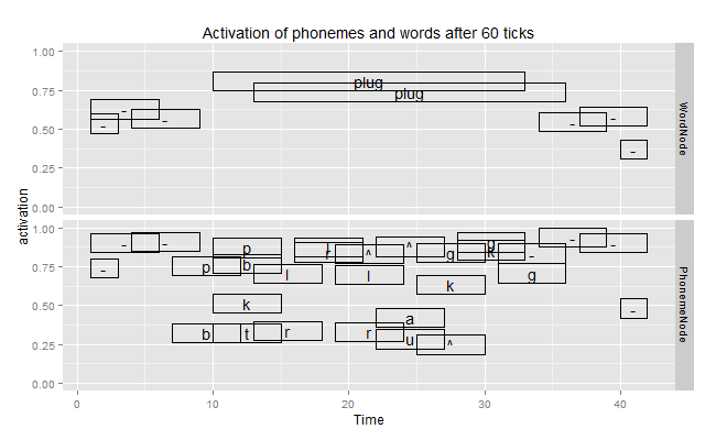
The above figure is from the Ganong effect demo in my report. It shows the activation of phonemes and word units over time when the network was presented with Xlug where “X” is an intermediate sound between /p/ and /b/. The network initially guesses blood and plug, but decides on plug once /g/ arrives. Afterwards, top-down connections from plug to /p/ cause activation for /p/ to rise above /b/. This phenomenon illustrates how top-down knowledge of words can resolve ambiguities in the speech signal.
Programming postmortem
I wrote a naive implementation for network units using message-passing object-oriented programming. Each network node is a bundle of data, and we send instructions (messages) to these nodes to tell them to collect input from neighboring nodes or to update their activation values.
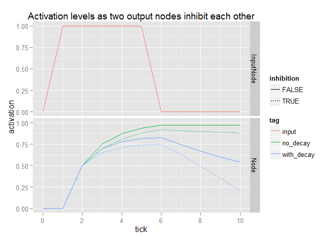
This implementation was partly inspired by Jeremy Kun’s implementation of backpropagation in Python. His implementation convinced me to start with a few nodes, make sure they behave as expected (see figure below), and bootstrap from there. And that’s how this implementation developed: I first created toy nodes to implement generic functionality, then figured out input nodes and feature detector nodes, wrote some functions to assemble a layer of those nodes, and then iterated to phoneme and word nodes/layers. Very interactive and organic, bootstrapped from the bottom up.
For the R programmers out there, I create the nodes as R6 objects. R
objects normally have copy-on-modify semantics so that when I
update x$value, I get a new copy of the object x. R6 objects have reference
semantics, meaning that they seal off a chunk of memory. I’m not sure why I
decided on R6 last year, but I probably reasoned that node$update() made more
sense than node <- update(node). I also convinced myself that R6 objects would
yield better performance because thousands of nodes wouldn’t have to be copied
on every network tick.
Unfortunately, the naive implementation doesn’t scale. When I tried to regenerate the plots yesterday, it took an hour for one network to complete 60 ticks. (I don’t remember it being that slow last year, but oh well.) I could try to optimize the pain away, but that would require profiling to find the pain points. Alternatively, I could ditch naive implementation and use a couple of data-frames: Store the nodes in a giant data-frame, and use split-apply-combine operations to e.g. summarize all the incoming activations to each node. Alternatively, I could keep the naive implementation but handle connections and activation calculations through matrix multiplication.
Papers as software documentation
My implementation was not a direct port of any other implementations. That is, I didn’t translate some source code into another language. Instead, I based my implementation on the description in the original paper. This top-down approach led to the most annoying part of the project.
Acoustic features like voiced, consonantal, vocalic, etc. are implemented in TRACE using values on a continuum from 1 to 8. A vowel sound like /a/ get s an 8 for vocalic, but a continuant sound like /s/ is kind of vocalic so it gets a value of 4. The original TRACE paper leads one to believe that each sound has just one value for each feature:
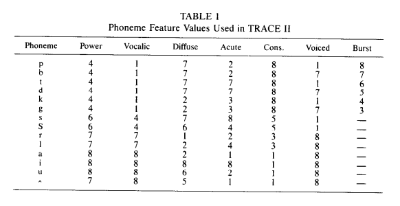
Based on the text, I implemented /k/’s acute feature as a vector [0, 0, 1, 0,
0, 0, 0, 0]. WRONG! That’s not what they did in 1986. The original C-TRACE
code defined the acute feature for /k/ as [.1, .3, 1, .3, .1, 0,
0, 0]. These smeared feature values popped up somewhere in the specs of each
phoneme, so all of my phoneme definitions were wrong. This mismatch between the
description in the paper and the original code caused a lot of headaches as my
simulations failed to obtain expected results. That was the most frustrating
part of the project, illustrating a disadvantage of my paper-first strategy of
implementating TRACE. A write-up can gloss over details, but the code doesn’t
lie.
Leave a comment