Recent adventures with lazyeval

The lazyeval package is a toolset for performing nonstandard evaluation in R. Nonstandard evaluation refers to any situation where something special happens with how user input or code is evaluated.

For example, the library() function doesn’t evaluate variables. In the example below, I try to trick library() into loading a fake package called evil_package by assigning to the package name lazyeval. In other words, we have the expression lazyeval and its value is "evil_package".

print(.packages())
#> [1] "knitr"     "stats"     "graphics"  "grDevices" "utils"     "datasets" 
#> [7] "methods"   "base"

lazyeval <- "evil_package"
library(lazyeval)

# The lazyeval package is loaded now.
print(.packages())
#> [1] "lazyeval"  "knitr"     "stats"     "graphics"  "grDevices" "utils"    
#> [7] "datasets"  "methods"   "base"

But this gambit doesn’t work because library() did something special: It didn’t evaluate the expression lazyeval. In the source code of library(), there is a line package <- as.character(substitute(package)) which replaces the value of package with a character version of the expression that the user wrote.

That’s a simple example of nonstandard evaluation, but it’s pervasive. It’s why you never have to quote column names in dplyr or ggplot2. In this post, I present some recent examples where I decided to use the lazyeval package to do something nonstandard. These examples are straight out of the lazyeval vignette in terms of complexity, but that’s fine. We all have to start somewhere.

Capturing expressions

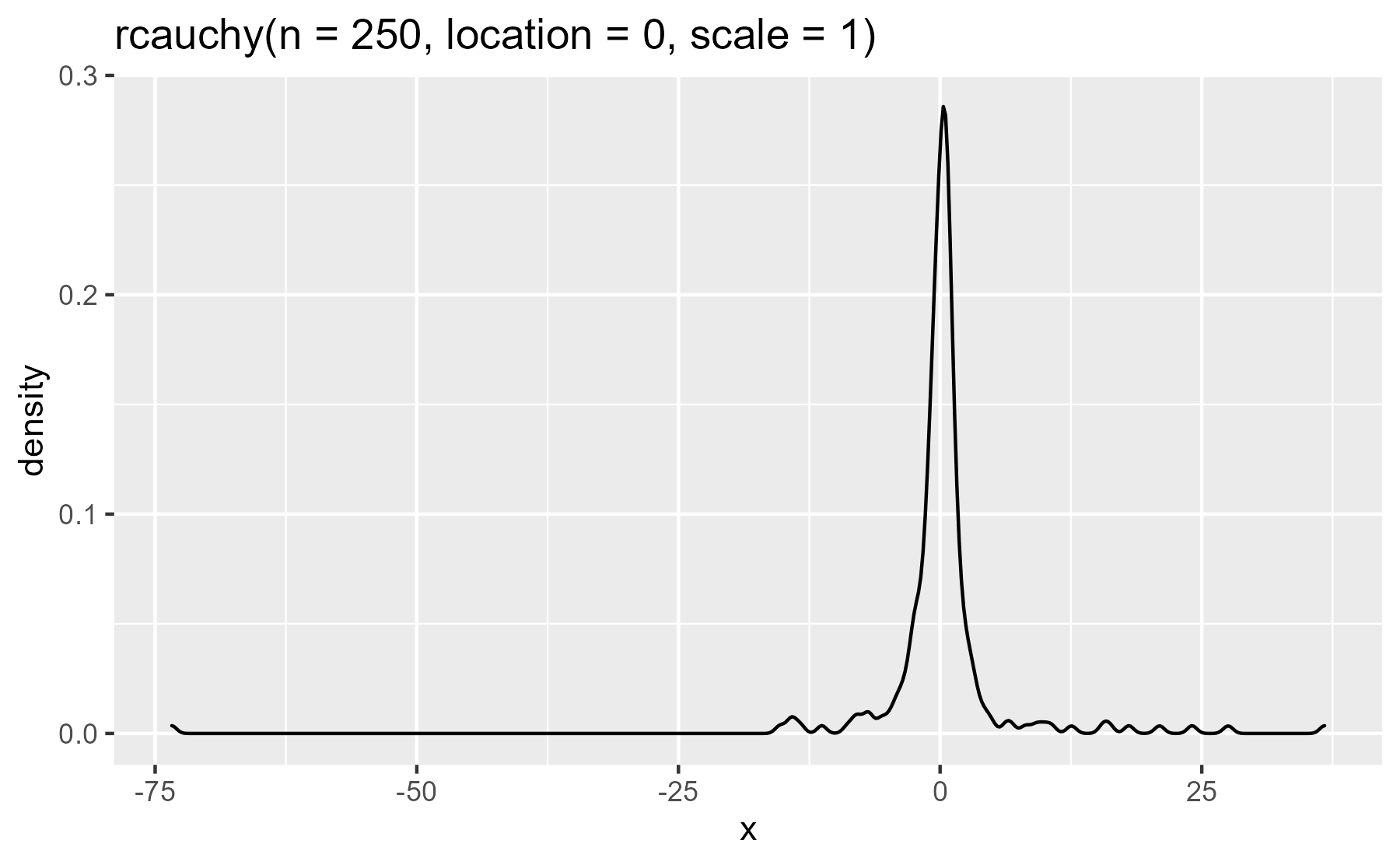
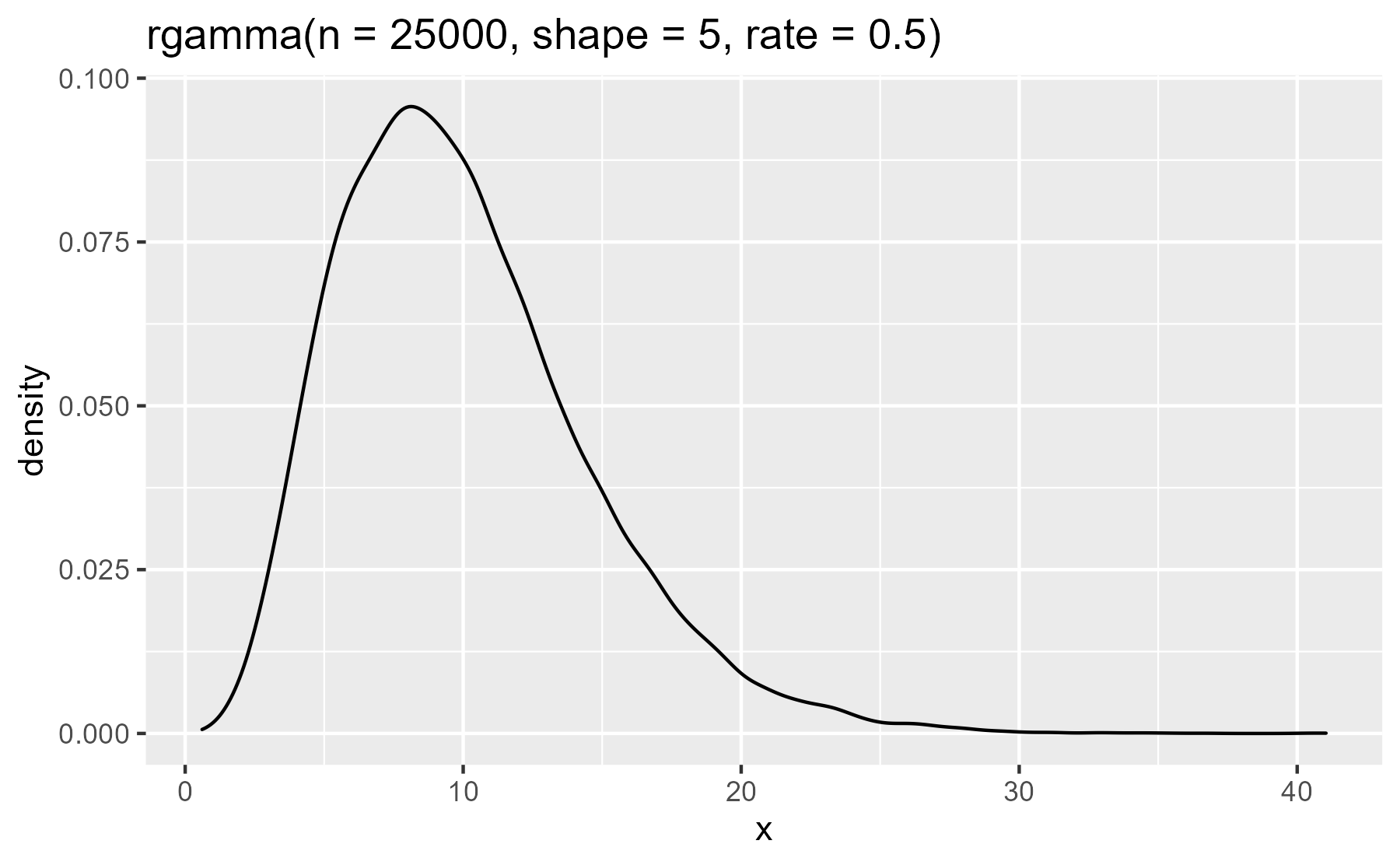
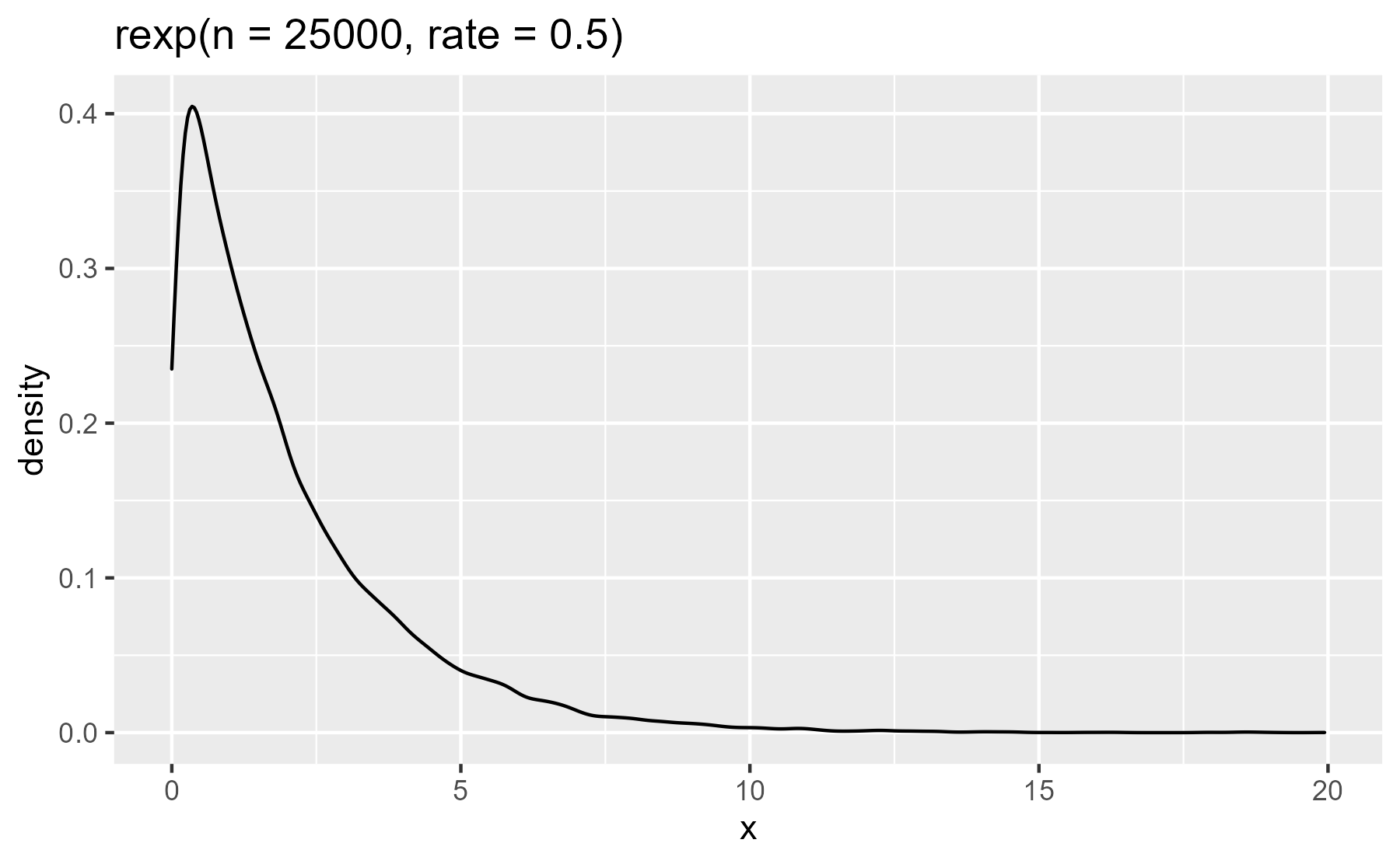
Plot titles. While reading the book Machine Learning For Hackers, I wanted to plot random numbers generated by probability distributions discussed by the book. I used the lazyeval::expr_text() function to capture the command used to generate the numbers and write it as the title of the plot.

library(dplyr, warn.conflicts = FALSE)
library(ggplot2)

plot_dist <- function(xs) {
  data <- tibble(x = xs)
  ggplot(data) +
    aes(x = x) +
    geom_density() +
    ggtitle(lazyeval::expr_text(xs)) 
}

plot_dist(rcauchy(n = 250, location = 0, scale = 1))

plot_dist(rgamma(n = 25000, shape = 5, rate = .5))

plot_dist(rexp(n = 25000, rate = .5))

Less fussy warning messages. I recently inherited some code where there were custom warning messages based on the input. The code threw a warning whenever a duplicate participant ID was found in a survey. It went something like this:

# some dummy data
study1 <- tibble(
  id = c(1, 2, 3, 4), 
  response = c("b", "c", "a", "b")
)

study2 <- tibble(
  id = c(1, 2, 2, 3, 1), 
  response = c("a", "a", "a", "b", "c")
)

if (anyDuplicated(study1$id)) {
  warning("Duplicate IDs found in Study1", call. = FALSE)
}

if (anyDuplicated(study2$id)) {
  warning("Duplicate IDs found in Study2", call. = FALSE)
}
#> Warning: Duplicate IDs found in Study2

To extend this code to a new study, one would just copy-and-paste and update the if statement’s condition and warning messages. Like so:

study3 <- tibble(
  id = c(1, 2, 3, 2), 
  response = c("b", "c", "a", "b")
)

if (anyDuplicated(study3$id)) {
  warning("Duplicate IDs found in Study2", call. = FALSE)
}
#> Warning: Duplicate IDs found in Study2

Wait, that’s not right! I forgot to update the warning message…

This setup is too brittle for me, so I abstracted the procedure into a function. First, I wrote a helper function to print out duplicates elements in a vector. This helper will let us make the warning message a little more informative.

# Print out duplicated elements in a vector
print_duplicates <- function(xs) {
  duplicated <- xs[duplicated(xs)]
  duplicated %>% sort() %>% unique() %>% paste0(collapse = ", ")
}

print_duplicates(study2$id)
#> [1] "1, 2"

Next, I wrote a function to issue the warnings. I used lazyeval::expr_label() convert the user-inputted expression into a string wrapped in backticks.

# Print a warning if duplicates are found in a vector
warn_duplicates <- function(xs) {
  if (anyDuplicated(xs)) {
    # Get what the user wrote for the xs argument
    actual_xs <- lazyeval::expr_label(xs)
    msg <- paste0(
      "Duplicate entries in ", actual_xs, ": ", print_duplicates(xs)
    )
    warning(msg, call. = FALSE)
  }
  invisible(NULL)
}

warn_duplicates(study1$id)
warn_duplicates(study2$id)
#> Warning: Duplicate entries in `study2$id`: 1, 2
warn_duplicates(study3$id)
#> Warning: Duplicate entries in `study3$id`: 2

The advantage of this approach is that the warning is a generic message that can work on any input. But in a funny way, the warning is also customized for the input because it includes the input printed verbatim.

An aside: In plotting, I used lazyeval::expr_text(), but here I used lazyeval::expr_label(). The two differ slightly. Namely, expr_label() surrounds the captured expression with backticks to indicate that expression is code:

lazyeval::expr_text(stop())
#> [1] "stop()"
lazyeval::expr_label(stop())
#> [1] "`stop()`"

# 2021-01-05: rlang requires you to separate the quoting from the quoting
rlang::quo_text(quote(stop()))
#> [1] "stop()"
rlang::quo_label(quote(stop()))
#> [1] "`stop()`"

rlang::quo_text(rlang::quo(stop()))
#> [1] "stop()"
rlang::quo_label(rlang::quo(stop()))
#> [1] "`stop()`"

Asking questions about a posterior distribution

I fit regression models with RStanARM. It lets me fit Bayesian models in Stan by writing conventional R modeling code. (Btw, I’m giving a tutorial on RStanARM in a month.)

Here’s a model about some famous flowers.

library(rstanarm)

model <- stan_glm(
  Petal.Width ~ Petal.Length * Species,
  data = iris,
  family = gaussian(), 
  prior = normal(0, 1)
)

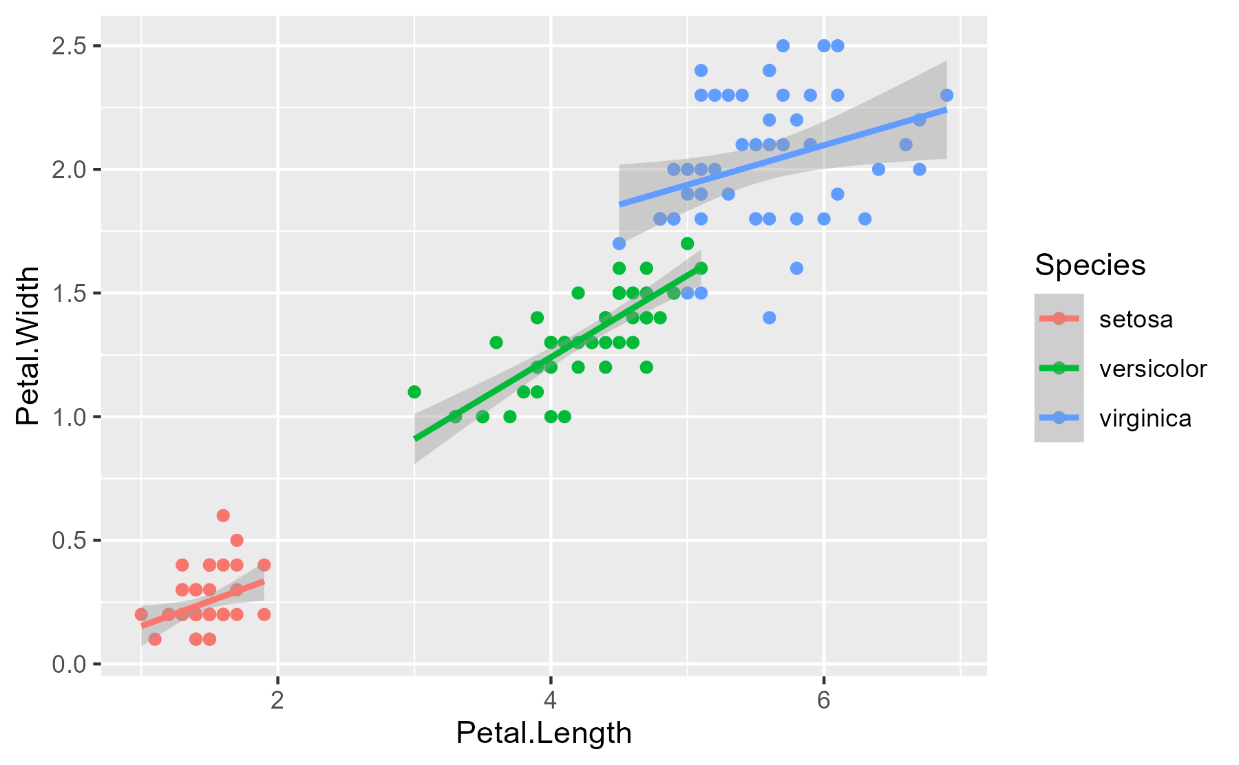
Here’s the essential relationship being explored.

ggplot(iris) + 
  aes(x = Petal.Length, y = Petal.Width, color = Species) + 
  geom_point() + 
  stat_smooth(method = "lm")
#> `geom_smooth()` using formula 'y ~ x'

The model gives me 4000 samples from the posterior distribution of the model.

summary(model)
#> 
#> Model Info:
#>  function:     stan_glm
#>  family:       gaussian [identity]
#>  formula:      Petal.Width ~ Petal.Length * Species
#>  algorithm:    sampling
#>  sample:       4000 (posterior sample size)
#>  priors:       see help('prior_summary')
#>  observations: 150
#>  predictors:   6
#> 
#> Estimates:
#>                                  mean   sd   10%   50%   90%
#> (Intercept)                     0.0    0.2 -0.3   0.0   0.3 
#> Petal.Length                    0.2    0.1  0.0   0.2   0.4 
#> Speciesversicolor              -0.1    0.3 -0.5  -0.1   0.3 
#> Speciesvirginica                1.1    0.3  0.7   1.1   1.5 
#> Petal.Length:Speciesversicolor  0.2    0.1  0.0   0.2   0.3 
#> Petal.Length:Speciesvirginica   0.0    0.1 -0.2   0.0   0.2 
#> sigma                           0.2    0.0  0.2   0.2   0.2 
#> 
#> Fit Diagnostics:
#>            mean   sd   10%   50%   90%
#> mean_PPD 1.2    0.0  1.2   1.2   1.2  
#> 
#> The mean_ppd is the sample average posterior predictive distribution of the outcome variable (for details see help('summary.stanreg')).
#> 
#> MCMC diagnostics
#>                                mcse Rhat n_eff
#> (Intercept)                    0.0  1.0   937 
#> Petal.Length                   0.0  1.0   949 
#> Speciesversicolor              0.0  1.0  1268 
#> Speciesvirginica               0.0  1.0  1238 
#> Petal.Length:Speciesversicolor 0.0  1.0   941 
#> Petal.Length:Speciesvirginica  0.0  1.0   874 
#> sigma                          0.0  1.0  2173 
#> mean_PPD                       0.0  1.0  3282 
#> log-posterior                  0.1  1.0  1251 
#> 
#> For each parameter, mcse is Monte Carlo standard error, n_eff is a crude measure of effective sample size, and Rhat is the potential scale reduction factor on split chains (at convergence Rhat=1).

At the 2.5% quantile, the Petal.Length effect looks like zero or less than zero. What proportion of the Petal.Length effects (for setosa flowers) is positive?

To answer questions like this one in a convenient way, I wrote a function that takes a boolean expression about a model’s parameters and evaluates it inside of the data-frame summary of the model posterior distribution. lazyeval::f_eval() does the nonstandard evaluation: It evaluates an expression captured by a formula like ~ 0 < Petal.Length inside of a list or data-frame. (Note that the mean of a logical vector is the proportion of the elements that are true.)

# Get proportion of posterior samples satisfying some inequality
posterior_proportion_ <- function(model, inequality) {
  draws <- as.data.frame(model)
  mean(lazyeval::f_eval(inequality, data = draws))
}

posterior_proportion_(model, ~ 0 < Petal.Length)
#> [1] 0.895

But all those tildes… The final underscore in posterior_proportion_() follows a convention for distinguishing between nonstandard evaluation functions that require formulas and those that do not. In the dplyr package, for example, there is select_()/select()/, mutate_()/mutate(), and so on. We can do the formula-free form of this function by using lazyeval::f_capture() to capture the input expression as a formula. We then hand that off to the version of the function that takes a formula.

posterior_proportion <- function(model, expr) {
  posterior_proportion_(model, lazyeval::f_capture(expr))
}

posterior_proportion(model, 0 < Petal.Length)
#> [1] 0.895

Here’s another question: What proportion of the posterior of the Petal.Length effect for virginica flowers is positive? In classical models, we would change the reference level for the categorical variable, refit the model, and check the significance. But I don’t want to refit this model because that would repeat the MCMC sampling. (It takes about 30 seconds to fit this model after all!) I’ll just ask the model for the sum of Petal.Length and Petal.Length:Speciesversicolor effects. That will give me the estimated Petal.Length effect but adjusted for the versicolor species.

posterior_proportion(model, 0 < Petal.Length + `Petal.Length:Speciesversicolor`)
#> [1] 1

posterior_proportion(model, 0 < Petal.Length + `Petal.Length:Speciesvirginica`)
#> [1] 1

(The backticks around Petal.Length:Speciesversicolor here prevent the : symbol from being evaluated as an operator.)

---

Last knitted on 2022-05-27. Source code on GitHub.¹

1. sessioninfo::session_info()
   #> ─ Session info ───────────────────────────────────────────────────────────────
   #>  setting  value
   #>  version  R version 4.2.0 (2022-04-22 ucrt)
   #>  os       Windows 10 x64 (build 22000)
   #>  system   x86_64, mingw32
   #>  ui       RTerm
   #>  language (EN)
   #>  collate  English_United States.utf8
   #>  ctype    English_United States.utf8
   #>  tz       America/Chicago
   #>  date     2022-05-27
   #>  pandoc   NA
   #> 
   #> ─ Packages ───────────────────────────────────────────────────────────────────
   #>  ! package      * version  date (UTC) lib source
   #>    assertthat     0.2.1    2019-03-21 [1] CRAN (R 4.2.0)
   #>    base64enc      0.1-3    2015-07-28 [1] CRAN (R 4.2.0)
   #>    bayesplot      1.9.0    2022-03-10 [1] CRAN (R 4.2.0)
   #>    boot           1.3-28   2021-05-03 [2] CRAN (R 4.2.0)
   #>    callr          3.7.0    2021-04-20 [1] CRAN (R 4.2.0)
   #>    cli            3.3.0    2022-04-25 [1] CRAN (R 4.2.0)
   #>    codetools      0.2-18   2020-11-04 [2] CRAN (R 4.2.0)
   #>    colorspace     2.0-3    2022-02-21 [1] CRAN (R 4.2.0)
   #>    colourpicker   1.1.1    2021-10-04 [1] CRAN (R 4.2.0)
   #>    crayon         1.5.1    2022-03-26 [1] CRAN (R 4.2.0)
   #>    crosstalk      1.2.0    2021-11-04 [1] CRAN (R 4.2.0)
   #>    DBI            1.1.2    2021-12-20 [1] CRAN (R 4.2.0)
   #>    digest         0.6.29   2021-12-01 [1] CRAN (R 4.2.0)
   #>    dplyr        * 1.0.9    2022-04-28 [1] CRAN (R 4.2.0)
   #>    DT             0.23     2022-05-10 [1] CRAN (R 4.2.0)
   #>    dygraphs       1.1.1.6  2018-07-11 [1] CRAN (R 4.2.0)
   #>    ellipsis       0.3.2    2021-04-29 [1] CRAN (R 4.2.0)
   #>    evaluate       0.15     2022-02-18 [1] CRAN (R 4.2.0)
   #>    fansi          1.0.3    2022-03-24 [1] CRAN (R 4.2.0)
   #>    farver         2.1.0    2021-02-28 [1] CRAN (R 4.2.0)
   #>    fastmap        1.1.0    2021-01-25 [1] CRAN (R 4.2.0)
   #>    generics       0.1.2    2022-01-31 [1] CRAN (R 4.2.0)
   #>    ggplot2      * 3.3.6    2022-05-03 [1] CRAN (R 4.2.0)
   #>    ggridges       0.5.3    2021-01-08 [1] CRAN (R 4.2.0)
   #>    git2r          0.30.1   2022-03-16 [1] CRAN (R 4.2.0)
   #>    glue           1.6.2    2022-02-24 [1] CRAN (R 4.2.0)
   #>    gridExtra      2.3      2017-09-09 [1] CRAN (R 4.2.0)
   #>    gtable         0.3.0    2019-03-25 [1] CRAN (R 4.2.0)
   #>    gtools         3.9.2.1  2022-05-23 [1] CRAN (R 4.2.0)
   #>    here           1.0.1    2020-12-13 [1] CRAN (R 4.2.0)
   #>    highr          0.9      2021-04-16 [1] CRAN (R 4.2.0)
   #>    htmltools      0.5.2    2021-08-25 [1] CRAN (R 4.2.0)
   #>    htmlwidgets    1.5.4    2021-09-08 [1] CRAN (R 4.2.0)
   #>    httpuv         1.6.5    2022-01-05 [1] CRAN (R 4.2.0)
   #>    igraph         1.3.1    2022-04-20 [1] CRAN (R 4.2.0)
   #>    inline         0.3.19   2021-05-31 [1] CRAN (R 4.2.0)
   #>    knitr        * 1.39     2022-04-26 [1] CRAN (R 4.2.0)
   #>    labeling       0.4.2    2020-10-20 [1] CRAN (R 4.2.0)
   #>    later          1.3.0    2021-08-18 [1] CRAN (R 4.2.0)
   #>    lattice        0.20-45  2021-09-22 [2] CRAN (R 4.2.0)
   #>    lazyeval     * 0.2.2    2019-03-15 [1] CRAN (R 4.2.0)
   #>    lifecycle      1.0.1    2021-09-24 [1] CRAN (R 4.2.0)
   #>    lme4           1.1-29   2022-04-07 [1] CRAN (R 4.2.0)
   #>    loo            2.5.1    2022-03-24 [1] CRAN (R 4.2.0)
   #>    magrittr       2.0.3    2022-03-30 [1] CRAN (R 4.2.0)
   #>    markdown       1.1      2019-08-07 [1] CRAN (R 4.2.0)
   #>    MASS           7.3-56   2022-03-23 [2] CRAN (R 4.2.0)
   #>    Matrix         1.4-1    2022-03-23 [2] CRAN (R 4.2.0)
   #>    matrixStats    0.62.0   2022-04-19 [1] CRAN (R 4.2.0)
   #>    mgcv           1.8-40   2022-03-29 [2] CRAN (R 4.2.0)
   #>    mime           0.12     2021-09-28 [1] CRAN (R 4.2.0)
   #>    miniUI         0.1.1.1  2018-05-18 [1] CRAN (R 4.2.0)
   #>    minqa          1.2.4    2014-10-09 [1] CRAN (R 4.2.0)
   #>    munsell        0.5.0    2018-06-12 [1] CRAN (R 4.2.0)
   #>    nlme           3.1-157  2022-03-25 [2] CRAN (R 4.2.0)
   #>    nloptr         2.0.2    2022-05-19 [1] CRAN (R 4.2.0)
   #>    pillar         1.7.0    2022-02-01 [1] CRAN (R 4.2.0)
   #>    pkgbuild       1.3.1    2021-12-20 [1] CRAN (R 4.2.0)
   #>    pkgconfig      2.0.3    2019-09-22 [1] CRAN (R 4.2.0)
   #>    plyr           1.8.7    2022-03-24 [1] CRAN (R 4.2.0)
   #>    prettyunits    1.1.1    2020-01-24 [1] CRAN (R 4.2.0)
   #>    processx       3.5.3    2022-03-25 [1] CRAN (R 4.2.0)
   #>    promises       1.2.0.1  2021-02-11 [1] CRAN (R 4.2.0)
   #>    ps             1.7.0    2022-04-23 [1] CRAN (R 4.2.0)
   #>    purrr          0.3.4    2020-04-17 [1] CRAN (R 4.2.0)
   #>    R6             2.5.1    2021-08-19 [1] CRAN (R 4.2.0)
   #>    ragg           1.2.2    2022-02-21 [1] CRAN (R 4.2.0)
   #>    Rcpp           1.0.8.3  2022-03-17 [1] CRAN (R 4.2.0)
   #>  D RcppParallel   5.1.5    2022-01-05 [1] CRAN (R 4.2.0)
   #>    reshape2       1.4.4    2020-04-09 [1] CRAN (R 4.2.0)
   #>    rlang          1.0.2    2022-03-04 [1] CRAN (R 4.2.0)
   #>    rprojroot      2.0.3    2022-04-02 [1] CRAN (R 4.2.0)
   #>    rstan          2.21.5   2022-04-11 [1] CRAN (R 4.2.0)
   #>    rstanarm       2.21.3   2022-04-09 [1] CRAN (R 4.2.0)
   #>    rstantools     2.2.0    2022-04-08 [1] CRAN (R 4.2.0)
   #>    rstudioapi     0.13     2020-11-12 [1] CRAN (R 4.2.0)
   #>    scales         1.2.0    2022-04-13 [1] CRAN (R 4.2.0)
   #>    sessioninfo    1.2.2    2021-12-06 [1] CRAN (R 4.2.0)
   #>    shiny          1.7.1    2021-10-02 [1] CRAN (R 4.2.0)
   #>    shinyjs        2.1.0    2021-12-23 [1] CRAN (R 4.2.0)
   #>    shinystan      2.6.0    2022-03-03 [1] CRAN (R 4.2.0)
   #>    shinythemes    1.2.0    2021-01-25 [1] CRAN (R 4.2.0)
   #>    StanHeaders    2.21.0-7 2020-12-17 [1] CRAN (R 4.2.0)
   #>    stringi        1.7.6    2021-11-29 [1] CRAN (R 4.2.0)
   #>    stringr        1.4.0    2019-02-10 [1] CRAN (R 4.2.0)
   #>    survival       3.3-1    2022-03-03 [2] CRAN (R 4.2.0)
   #>    systemfonts    1.0.4    2022-02-11 [1] CRAN (R 4.2.0)
   #>    textshaping    0.3.6    2021-10-13 [1] CRAN (R 4.2.0)
   #>    threejs        0.3.3    2020-01-21 [1] CRAN (R 4.2.0)
   #>    tibble         3.1.7    2022-05-03 [1] CRAN (R 4.2.0)
   #>    tidyselect     1.1.2    2022-02-21 [1] CRAN (R 4.2.0)
   #>    utf8           1.2.2    2021-07-24 [1] CRAN (R 4.2.0)
   #>    vctrs          0.4.1    2022-04-13 [1] CRAN (R 4.2.0)
   #>    withr          2.5.0    2022-03-03 [1] CRAN (R 4.2.0)
   #>    xfun           0.31     2022-05-10 [1] CRAN (R 4.2.0)
   #>    xtable         1.8-4    2019-04-21 [1] CRAN (R 4.2.0)
   #>    xts            0.12.1   2020-09-09 [1] CRAN (R 4.2.0)
   #>    zoo            1.8-10   2022-04-15 [1] CRAN (R 4.2.0)
   #> 
   #>  [1] C:/Users/Tristan/AppData/Local/R/win-library/4.2
   #>  [2] C:/Program Files/R/R-4.2.0/library
   #> 
   #>  D ── DLL MD5 mismatch, broken installation.
   #> 
   #> ──────────────────────────────────────────────────────────────────────────────
   

   ↩