Simplifying ggplot2 code by doing nothing
Recently, I joined the development team for bayesplot, an R package by the Stan team for plotting Bayesian models. Because visualizing Bayesian models in ggplot2 is a recurring topic here, it was a natural fit. So from time to time, I’ll post about some programming techniques and new features we develop in the bayesplot package.
For this post, I describe one of strategies I have been using to clean up and simplify some of the plotting code in the package: avoid if-branches by sometimes plotting nothing.
Warm-up example
Let’s start with a non-plotting example. We consider a function that takes a list of counts of people and returns the total number of people. That sum, however, is controlled by some of the function’s arguments:
library(magrittr)
head_count <- function(data, staff = FALSE, faculty = FALSE) {
  total <- data[["students"]]

  if (staff) {
    total <- total + data[["staff"]]
  }

  if (faculty) {
    total <- total + data[["faculty"]]
  }

  total
}

data <- list(students = 10, staff = 3, faculty = 2)
head_count(data)
#> [1] 10
head_count(data, staff = TRUE)
#> [1] 13
head_count(data, faculty = TRUE)
#> [1] 12
The function as it’s written works fine… but the if-branches get in the
way. The main job of the function is to assemble something (a sum) from
pieces of data, but that assembly is split across the if-branches. The total
is updated in-place twice (total <- total + ...). I would rather combine all
the data in one fell swoop.
One way to move the data-assembly out of these if-branches is to make the data
conditional. That is, instead of doing the addition in the if statements, we
do all the addition at once but just add 0 when a piece of data isn’t
needed. This technique simplifies the function definition:
head_count <- function(data, staff = FALSE, faculty = FALSE) {
  staff <- if (staff) data[["staff"]] else 0
  faculty <- if (faculty) data[["faculty"]] else 0

  data[["students"]] + staff + faculty
}

head_count(data)
#> [1] 10
head_count(data, staff = TRUE)
#> [1] 13
head_count(data, faculty = TRUE)
#> [1] 12
For operations where we combine things to get a new thing, there’s often an identity element: a value we can plug in as a placeholder value without changing the results. Some examples:
# multiplication
pi * 1
#> [1] 3.141593

# string concatenation
paste0("a", "")
#> [1] "a"

# combining things
c(1, 2, 3, c())
#> [1] 1 2 3

# data-frame binding
rbind(head(iris), list())
#>   Sepal.Length Sepal.Width Petal.Length Petal.Width Species
#> 1          5.1         3.5          1.4         0.2  setosa
#> 2          4.9         3.0          1.4         0.2  setosa
#> 3          4.7         3.2          1.3         0.2  setosa
#> 4          4.6         3.1          1.5         0.2  setosa
#> 5          5.0         3.6          1.4         0.2  setosa
#> 6          5.4         3.9          1.7         0.4  setosa

# magrittr pipes
f <- function(x, ...) x
1:2 %>% f()
#> [1] 1 2
Below, I demonstrate two examples of how I applied a similar strategy in
bayesplot. In ggplot2, we assemble plots by adding layers and options to a plot
by stringing together statements with +. To handle conditional plotting
elements and construct the plot all in one pass, I took advantage of ways to
adding nothing to a ggplot2 plot.1
Posterior interval plots
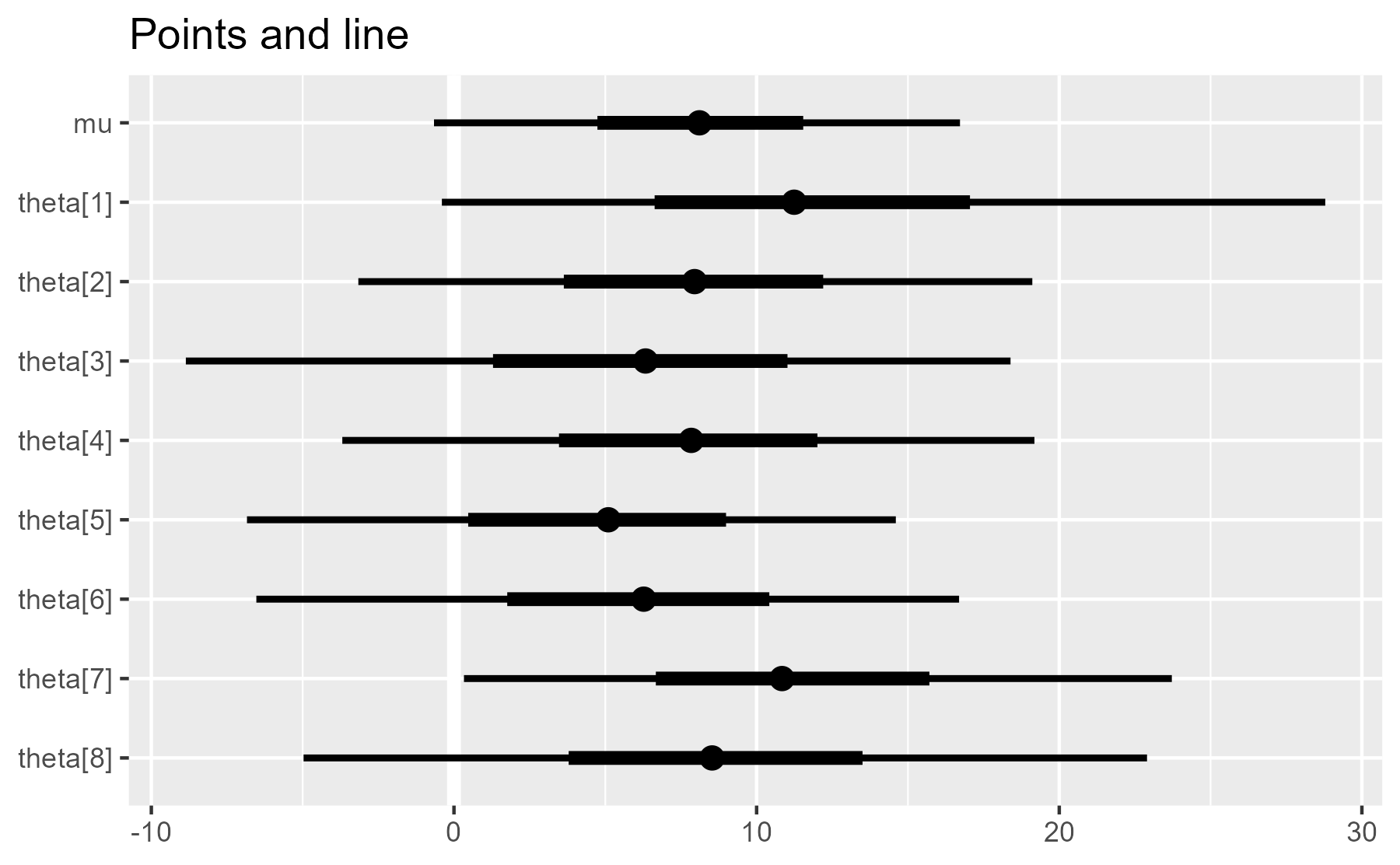
Here are some posterior samples for a Bayesian model, in this case the “eight schools” meta-analysis example. We want to create a plot that shows the 90% and 50% uncertainty intervals for each parameter.
We first use a helper function to clean up the data to prepare it for plotting.
(At the time of writing, mcmc_intervals_data() is not yet in the CRAN version
of bayesplot.)
library(dplyr, warn.conflicts = FALSE)
library(bayesplot)
#> This is bayesplot version 1.9.0
#> - Online documentation and vignettes at mc-stan.org/bayesplot
#> - bayesplot theme set to bayesplot::theme_default()
#>    * Does _not_ affect other ggplot2 plots
#>    * See ?bayesplot_theme_set for details on theme setting
library(ggplot2)
theme_set(theme_grey())

interval_data <- shinystan::eight_schools@posterior_sample %>%
  mcmc_intervals_data(pars = "mu", regex_pars = "theta") %>%
  mutate_if(is.numeric, round, 2)

interval_data
#> # A tibble: 9 × 9
#>   parameter outer_width inner_width point_est    ll     l     m     h    hh
#>   <fct>           <dbl>       <dbl> <chr>     <dbl> <dbl> <dbl> <dbl> <dbl>
#> 1 mu                0.9         0.5 median    -0.66  4.74  8.11 11.5   16.7
#> 2 theta[1]          0.9         0.5 median    -0.4   6.63 11.2  17.0   28.8
#> 3 theta[2]          0.9         0.5 median    -3.16  3.63  7.95 12.2   19.1
#> 4 theta[3]          0.9         0.5 median    -8.86  1.29  6.33 11.0   18.4
#> 5 theta[4]          0.9         0.5 median    -3.69  3.47  7.84 12.0   19.2
#> 6 theta[5]          0.9         0.5 median    -6.84  0.47  5.1   8.99  14.6
#> 7 theta[6]          0.9         0.5 median    -6.53  1.76  6.27 10.4   16.7
#> 8 theta[7]          0.9         0.5 median     0.33  6.67 10.8  15.7   23.7
#> 9 theta[8]          0.9         0.5 median    -4.97  3.79  8.53 13.5   22.9
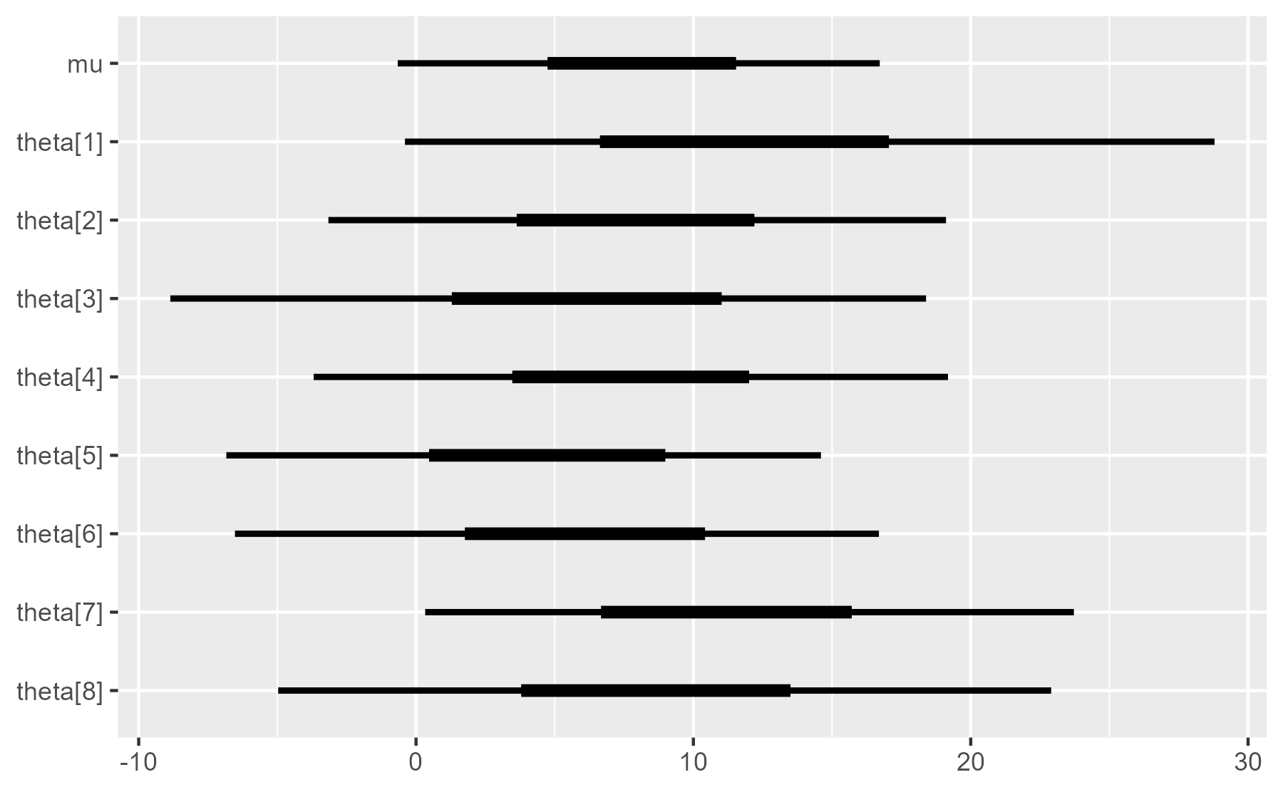
Below is the basic plot we want to
create. (Normally, in bayesplot, we would use
mcmc_intervals()
to make this plot, but for the sake of illustration, we will write a version of
it from scratch.
ggplot(interval_data) +
  aes_(y = ~ parameter, yend = ~ parameter) +
  geom_segment(aes_(x = ~ ll, xend = ~ hh), size = 1) +
  geom_segment(aes_(x = ~ l, xend = ~ h), size = 2) +
  scale_y_discrete(limits = rev(interval_data$parameter)) +
  labs(x = NULL, y = NULL)
Wait, what’s going on with the tildes? We use aes_(y = ~ parameter)
because in an R package, writing aes(y = parameter) would raise an undefined
global variable warning :warning: during CRAN package checks. The code looks like it uses
a variable called parameter, but a variable with that name has not been defined in
the code yet. The formula form ~ parameter “quotes” the variable name, so
it doesn’t appear as a global variable.
We are going to wrap this code in an R function along with two annotation options:
- whether to draw point estimates (medians) over the intervals
- whether to draw a vertical reference line at x = 0
Here is how we might write the function with branching code.
plot_intervals <- function(
  data,
  draw_points = TRUE,
  draw_ref_line = TRUE,
  line_position = 0
) {
  p <- ggplot(data) +
    aes_(y = ~ parameter, yend = ~ parameter)

  if (draw_ref_line) {
    p <- p +
      geom_vline(xintercept = line_position, size = 2, color = "white")
  }

  p <- p +
    geom_segment(aes_(x = ~ ll, xend = ~ hh), size = 1) +
    geom_segment(aes_(x = ~ l, xend = ~ h), size = 2)

  if (draw_points) {
    p <- p + geom_point(aes_(x = ~ m), size = 3)
  }

   p +
     scale_y_discrete(limits = rev(data$parameter)) +
     labs(x = NULL, y = NULL)
}

# Test the code
plot_intervals(interval_data) + ggtitle("Points and line")
plot_intervals(interval_data, draw_points = FALSE) + ggtitle("No points")
plot_intervals(interval_data, draw_ref_line = FALSE) + ggtitle("No line")

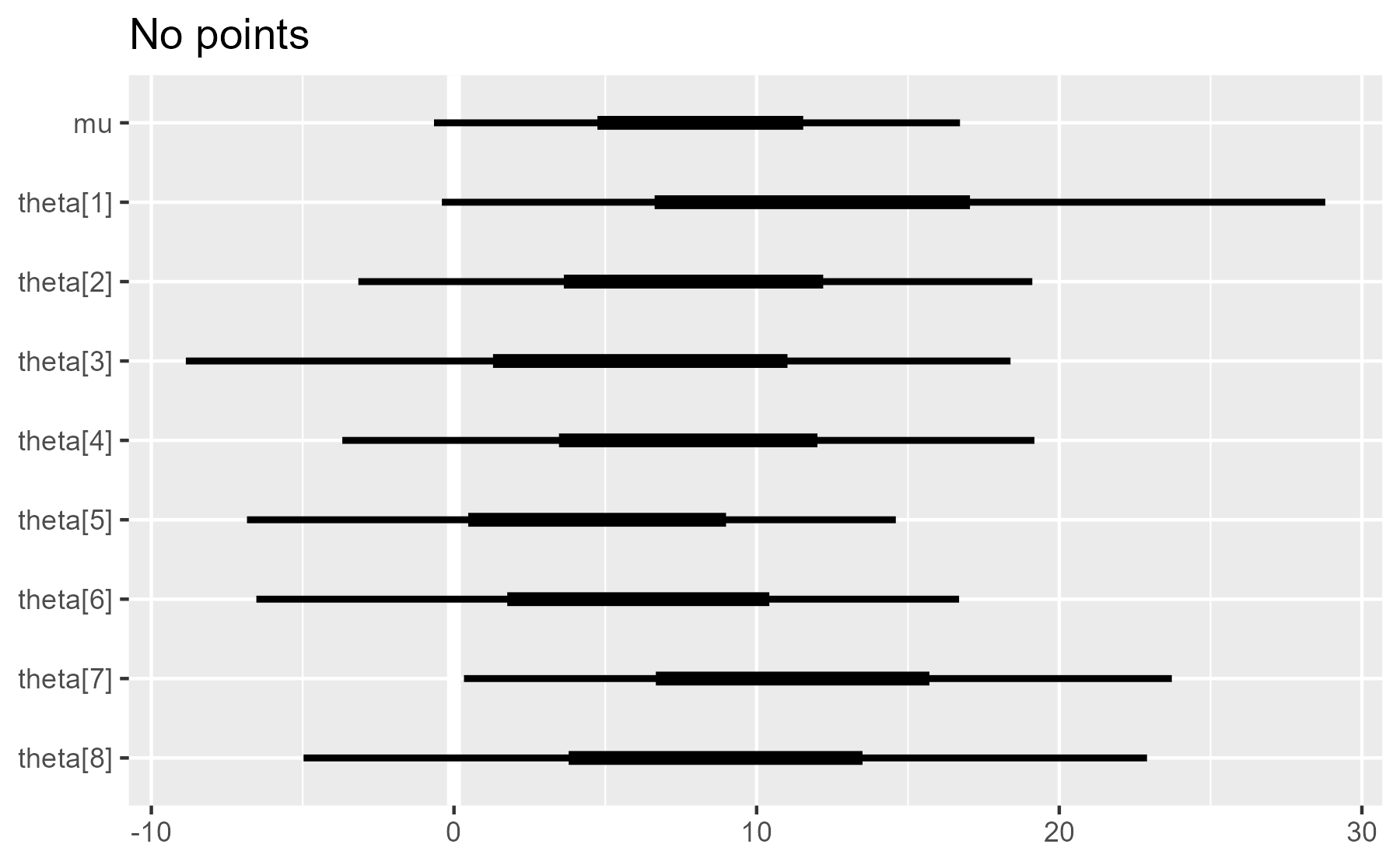
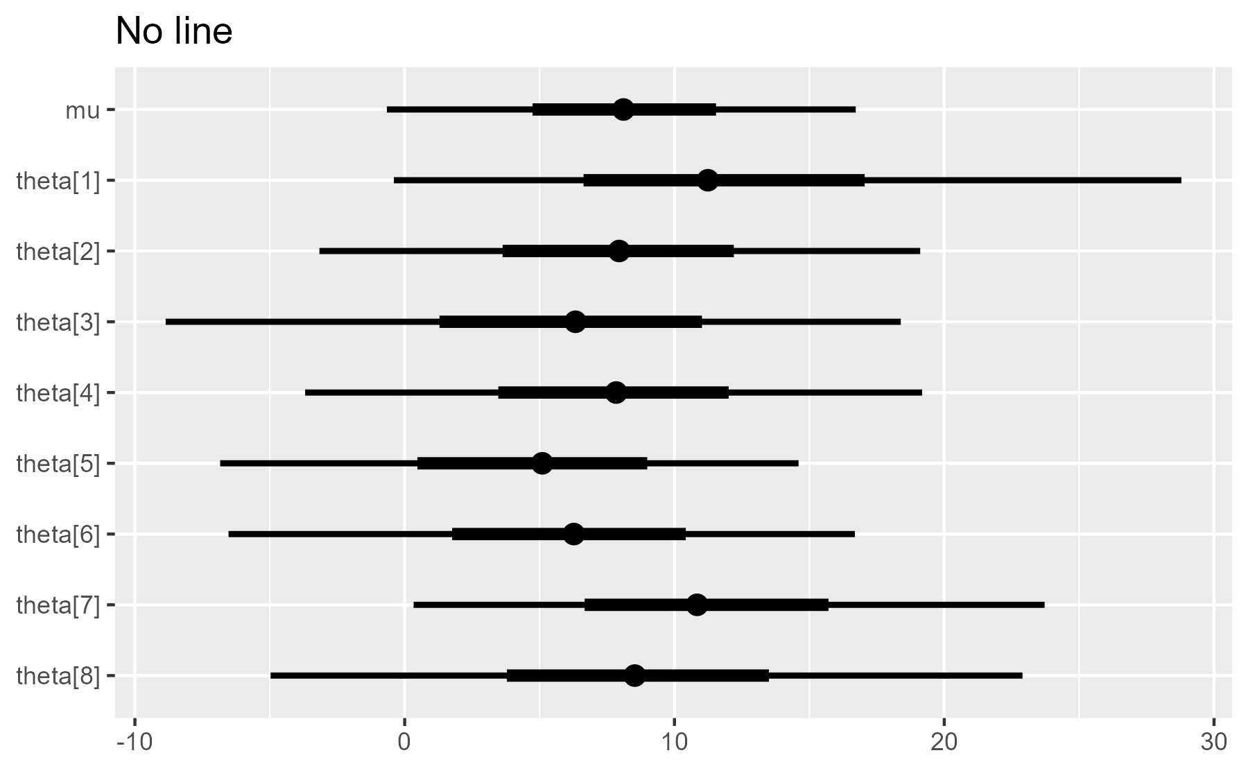
As we can see, the plot is built up incrementally throughout the function.
The plot object p is updated three times (the p <- p + ... parts). This
makes it more difficult to understand the function when reading it and increases
the chance that we might do something wrong when working on this code.
We can improve the readability by using empty or placeholder elements to move the plot updates outside of the if-branches.
Do nothing by plotting an empty dataframe
ggplot2 is built to work on dataframe columns, and if there is no data in a
column, it will quietly plot nothing. Therefore, one way to do nothing is to run
the normal geom_ plotting function but on an empty dataframe. Here, we apply
that strategy for the point estimates by toggling between the original data or
zero-row alternative in the first line.
plot_intervals <- function(
  data,
  draw_points = TRUE,
  draw_ref_line = TRUE,
  line_position = 0
) {
  maybe_points <- if (draw_points) data else data[0, ]

  p <- ggplot(data) +
    aes_(y = ~ parameter, yend = ~ parameter)

  if (draw_ref_line) {
    p <- p +
      geom_vline(xintercept = line_position, size = 2, color = "white")
  }

  p +
    geom_segment(aes_(x = ~ ll, xend = ~ hh), size = 1) +
    geom_segment(aes_(x = ~ l, xend = ~ h), size = 2) +
    geom_point(aes_(x = ~ m), data = maybe_points, size = 3) +
    scale_y_discrete(limits = rev(data$parameter)) +
    labs(x = NULL, y = NULL)
}

# Test the code
plot_intervals(interval_data) + ggtitle("Points and line")
plot_intervals(interval_data, draw_points = FALSE) + ggtitle("No points")


This is a marked improvement over the original, as most of the plot construction happens at the end of the function.
Do nothing with geom_blank()
Another way to do nothing is to add geom_blank(). In fact, this is what
ggplot2 does when we print a ggplot2 object without any geom layers.
ggplot(interval_data) +
  aes(x = m, y = parameter)
When we inspect the last plot that was displayed, we see geom_blank() is one
of the layers:
last_plot()[["layers"]]
#> [[1]]
#> geom_blank: na.rm = FALSE
#> stat_identity: na.rm = FALSE
#> position_identity
As a first pass for technique, we toggle between the plotting functions
geom_vline() and geom_blank(). This version simplifies the plot
construction to a single stream of plot additions.
plot_intervals <- function(
  data,
  draw_points = TRUE,
  draw_ref_line = TRUE,
  line_position = 0
) {
  maybe_points <- if (draw_points) data else data[0, ]
  geom_maybe_vline <- if (draw_ref_line) geom_vline else geom_blank

  ggplot(data) +
    aes_(y = ~ parameter, yend = ~ parameter) +
    geom_maybe_vline(xintercept = line_position, size = 2, color = "white") +
    geom_segment(aes_(x = ~ ll, xend = ~ hh), size = 1) +
    geom_segment(aes_(x = ~ l, xend = ~ h), size = 2) +
    geom_point(aes_(x = ~ m), data = maybe_points, size = 3) +
    scale_y_discrete(limits = rev(data$parameter)) +
    labs(x = NULL, y = NULL)
}

# Test the code
plot_intervals(interval_data) + ggtitle("Points and line")
plot_intervals(interval_data, draw_ref_line = FALSE) + ggtitle("No line")
#> Warning: Ignoring unknown parameters: xintercept, size, colour


But it also issues a warning when it toggles to geom_blank(). That might alarm
some users, so we need to fix that. For bayesplot, I wrote a helper called
geom_ignore() as a version of geom_blank() that ignores any input arguments.
The function receives any number of arguments in the ... placeholder argument,
but the function does nothing with those dots. It just ignores them.
geom_ignore <- function(...) {
  geom_blank(
    mapping = NULL,
    data = NULL,
    show.legend = FALSE,
    inherit.aes = FALSE
  )
}
For completeness, here is the final form using geom_ignore().
plot_intervals <- function(
  data,
  draw_points = TRUE,
  draw_ref_line = TRUE,
  line_position = 0
) {
  maybe_points <- if (draw_points) data else data[0, ]
  geom_maybe_vline <- if (draw_ref_line) geom_vline else geom_ignore

  ggplot(data) +
    aes_(y = ~ parameter, yend = ~ parameter) +
    geom_maybe_vline(xintercept = line_position, size = 2, color = "white") +
    geom_segment(aes_(x = ~ ll, xend = ~ hh), size = 1) +
    geom_segment(aes_(x = ~ l, xend = ~ h), size = 2) +
    geom_point(aes_(x = ~ m), data = maybe_points, size = 3) +
    scale_y_discrete(limits = rev(data$parameter)) +
    labs(x = NULL, y = NULL)
}

# Test the code
plot_intervals(interval_data) + ggtitle("Points and line")
plot_intervals(interval_data, draw_ref_line = FALSE) + ggtitle("No line")

A final note on NULL [updated]
I should come clean and note that these blank layers are not really identity
elements. Unlike adding 0 to a number, using these techniques to add nothing to
a plot still updates the plot’s data. For the plot object below, the first layer
says geom_blank and the last layer says geom_point. Visually, we have done
nothing, but internally, we left a trace behind.
p <- plot_intervals(
  interval_data,
  draw_points = FALSE,
  draw_ref_line = FALSE
)

p[["layers"]][[1]]
#> geom_blank: na.rm = FALSE
#> stat_identity: na.rm = FALSE
#> position_identity

p[["layers"]][[4]]
#> mapping: x = ~m
#> geom_point: na.rm = FALSE
#> stat_identity: na.rm = FALSE
#> position_identity
Update After some playing around, I discovered that adding NULL to
a ggplot doesn’t change it (e.g., p + NULL does not leave a trace), so
it provides a stronger identity element for ggplot2 than invisible
layers. In the original version of this post, I said that I would not
use NULL in this way because it seemed like an edge case that might
break some day. But the creator of ggplot2, Hadley Wickham, told me
that using NULL as an identity element is a deliberate design
feature.
🎉 Cool! Now, we can make geom_ignore() even
simpler.
geom_ignore <- function(...) {
  NULL
}
Last knitted on 2022-05-27. Source code on GitHub.2
-
This technique of using an empty element with combiner functions was inspired by the concept of monoids which come up in functional programming. Monoids have a strict formal definition, and ggplot2 are certainly not monoids because everything must be added onto an initial
ggplot()object. ↩ -
.session_info
#> ─ Session info ───────────────────────────────────────────────────────────────
#>  setting      value
#>  version      R version 4.2.0 (2022-04-22 ucrt)
#>  os           Windows 10 x64 (build 22000)
#>  system       x86_64, mingw32
#>  ui           RTerm
#>  language     (EN)
#>  collate      English_United States.utf8
#>  ctype        English_United States.utf8
#>  tz           America/Chicago
#>  date         2022-05-27
#>  pandoc       NA
#>  stan (rstan) 2.21.0
#>
#> ─ Packages ───────────────────────────────────────────────────────────────────
#>  ! package        * version    date (UTC) lib source
#>    abind            1.4-5      2016-07-21 [1] CRAN (R 4.2.0)
#>    assertthat       0.2.1      2019-03-21 [1] CRAN (R 4.2.0)
#>    backports        1.4.1      2021-12-13 [1] CRAN (R 4.2.0)
#>    base64enc        0.1-3      2015-07-28 [1] CRAN (R 4.2.0)
#>    bayesplot      * 1.9.0      2022-03-10 [1] CRAN (R 4.2.0)
#>    callr            3.7.0      2021-04-20 [1] CRAN (R 4.2.0)
#>    checkmate        2.1.0      2022-04-21 [1] CRAN (R 4.2.0)
#>    cli              3.3.0      2022-04-25 [1] CRAN (R 4.2.0)
#>    codetools        0.2-18     2020-11-04 [2] CRAN (R 4.2.0)
#>    colorspace       2.0-3      2022-02-21 [1] CRAN (R 4.2.0)
#>    colourpicker     1.1.1      2021-10-04 [1] CRAN (R 4.2.0)
#>    crayon           1.5.1      2022-03-26 [1] CRAN (R 4.2.0)
#>    crosstalk        1.2.0      2021-11-04 [1] CRAN (R 4.2.0)
#>    DBI              1.1.2      2021-12-20 [1] CRAN (R 4.2.0)
#>    digest           0.6.29     2021-12-01 [1] CRAN (R 4.2.0)
#>    distributional   0.3.0      2022-01-05 [1] CRAN (R 4.2.0)
#>    dplyr          * 1.0.9      2022-04-28 [1] CRAN (R 4.2.0)
#>    DT               0.23       2022-05-10 [1] CRAN (R 4.2.0)
#>    dygraphs         1.1.1.6    2018-07-11 [1] CRAN (R 4.2.0)
#>    ellipsis         0.3.2      2021-04-29 [1] CRAN (R 4.2.0)
#>    emo              0.0.0.9000 2022-05-25 [1] Github (hadley/emo@3f03b11)
#>    evaluate         0.15       2022-02-18 [1] CRAN (R 4.2.0)
#>    fansi            1.0.3      2022-03-24 [1] CRAN (R 4.2.0)
#>    farver           2.1.0      2021-02-28 [1] CRAN (R 4.2.0)
#>    fastmap          1.1.0      2021-01-25 [1] CRAN (R 4.2.0)
#>    generics         0.1.2      2022-01-31 [1] CRAN (R 4.2.0)
#>    ggplot2        * 3.3.6      2022-05-03 [1] CRAN (R 4.2.0)
#>    ggridges         0.5.3      2021-01-08 [1] CRAN (R 4.2.0)
#>    git2r            0.30.1     2022-03-16 [1] CRAN (R 4.2.0)
#>    glue             1.6.2      2022-02-24 [1] CRAN (R 4.2.0)
#>    gridExtra        2.3        2017-09-09 [1] CRAN (R 4.2.0)
#>    gtable           0.3.0      2019-03-25 [1] CRAN (R 4.2.0)
#>    gtools           3.9.2.1    2022-05-23 [1] CRAN (R 4.2.0)
#>    here             1.0.1      2020-12-13 [1] CRAN (R 4.2.0)
#>    highr            0.9        2021-04-16 [1] CRAN (R 4.2.0)
#>    htmltools        0.5.2      2021-08-25 [1] CRAN (R 4.2.0)
#>    htmlwidgets      1.5.4      2021-09-08 [1] CRAN (R 4.2.0)
#>    httpuv           1.6.5      2022-01-05 [1] CRAN (R 4.2.0)
#>    igraph           1.3.1      2022-04-20 [1] CRAN (R 4.2.0)
#>    inline           0.3.19     2021-05-31 [1] CRAN (R 4.2.0)
#>    knitr          * 1.39       2022-04-26 [1] CRAN (R 4.2.0)
#>    labeling         0.4.2      2020-10-20 [1] CRAN (R 4.2.0)
#>    later            1.3.0      2021-08-18 [1] CRAN (R 4.2.0)
#>    lattice          0.20-45    2021-09-22 [2] CRAN (R 4.2.0)
#>    lifecycle        1.0.1      2021-09-24 [1] CRAN (R 4.2.0)
#>    loo              2.5.1      2022-03-24 [1] CRAN (R 4.2.0)
#>    lubridate        1.8.0      2021-10-07 [1] CRAN (R 4.2.0)
#>    magrittr       * 2.0.3      2022-03-30 [1] CRAN (R 4.2.0)
#>    markdown         1.1        2019-08-07 [1] CRAN (R 4.2.0)
#>    matrixStats      0.62.0     2022-04-19 [1] CRAN (R 4.2.0)
#>    mime             0.12       2021-09-28 [1] CRAN (R 4.2.0)
#>    miniUI           0.1.1.1    2018-05-18 [1] CRAN (R 4.2.0)
#>    munsell          0.5.0      2018-06-12 [1] CRAN (R 4.2.0)
#>    pillar           1.7.0      2022-02-01 [1] CRAN (R 4.2.0)
#>    pkgbuild         1.3.1      2021-12-20 [1] CRAN (R 4.2.0)
#>    pkgconfig        2.0.3      2019-09-22 [1] CRAN (R 4.2.0)
#>    plyr             1.8.7      2022-03-24 [1] CRAN (R 4.2.0)
#>    posterior        1.2.1      2022-03-07 [1] CRAN (R 4.2.0)
#>    prettyunits      1.1.1      2020-01-24 [1] CRAN (R 4.2.0)
#>    processx         3.5.3      2022-03-25 [1] CRAN (R 4.2.0)
#>    promises         1.2.0.1    2021-02-11 [1] CRAN (R 4.2.0)
#>    ps               1.7.0      2022-04-23 [1] CRAN (R 4.2.0)
#>    purrr            0.3.4      2020-04-17 [1] CRAN (R 4.2.0)
#>    R6               2.5.1      2021-08-19 [1] CRAN (R 4.2.0)
#>    ragg             1.2.2      2022-02-21 [1] CRAN (R 4.2.0)
#>    Rcpp             1.0.8.3    2022-03-17 [1] CRAN (R 4.2.0)
#>  D RcppParallel     5.1.5      2022-01-05 [1] CRAN (R 4.2.0)
#>    reshape2         1.4.4      2020-04-09 [1] CRAN (R 4.2.0)
#>    rlang            1.0.2      2022-03-04 [1] CRAN (R 4.2.0)
#>    rprojroot        2.0.3      2022-04-02 [1] CRAN (R 4.2.0)
#>    rstan            2.21.5     2022-04-11 [1] CRAN (R 4.2.0)
#>    rstudioapi       0.13       2020-11-12 [1] CRAN (R 4.2.0)
#>    scales           1.2.0      2022-04-13 [1] CRAN (R 4.2.0)
#>    sessioninfo      1.2.2      2021-12-06 [1] CRAN (R 4.2.0)
#>    shiny            1.7.1      2021-10-02 [1] CRAN (R 4.2.0)
#>    shinyjs          2.1.0      2021-12-23 [1] CRAN (R 4.2.0)
#>    shinystan        2.6.0      2022-03-03 [1] CRAN (R 4.2.0)
#>    shinythemes      1.2.0      2021-01-25 [1] CRAN (R 4.2.0)
#>    StanHeaders      2.21.0-7   2020-12-17 [1] CRAN (R 4.2.0)
#>    stringi          1.7.6      2021-11-29 [1] CRAN (R 4.2.0)
#>    stringr          1.4.0      2019-02-10 [1] CRAN (R 4.2.0)
#>    systemfonts      1.0.4      2022-02-11 [1] CRAN (R 4.2.0)
#>    tensorA          0.36.2     2020-11-19 [1] CRAN (R 4.2.0)
#>    textshaping      0.3.6      2021-10-13 [1] CRAN (R 4.2.0)
#>    threejs          0.3.3      2020-01-21 [1] CRAN (R 4.2.0)
#>    tibble           3.1.7      2022-05-03 [1] CRAN (R 4.2.0)
#>    tidyselect       1.1.2      2022-02-21 [1] CRAN (R 4.2.0)
#>    utf8             1.2.2      2021-07-24 [1] CRAN (R 4.2.0)
#>    vctrs            0.4.1      2022-04-13 [1] CRAN (R 4.2.0)
#>    withr            2.5.0      2022-03-03 [1] CRAN (R 4.2.0)
#>    xfun             0.31       2022-05-10 [1] CRAN (R 4.2.0)
#>    xtable           1.8-4      2019-04-21 [1] CRAN (R 4.2.0)
#>    xts              0.12.1     2020-09-09 [1] CRAN (R 4.2.0)
#>    zoo              1.8-10     2022-04-15 [1] CRAN (R 4.2.0)
#>
#>  [1] C:/Users/Tristan/AppData/Local/R/win-library/4.2
#>  [2] C:/Program Files/R/R-4.2.0/library
#>
#>  D ── DLL MD5 mismatch, broken installation.
#>
#> ──────────────────────────────────────────────────────────────────────────────

Leave a comment